

Subjects
28 healthy volunteers (12 male and 16 females; mean age 25.7 years [24.1–27.4]; median body mass index (BMI) 21.5 kg/m² [IQR: 19.8–23.7]) who had signed informed consent were enrolled in the study. The study was approved by the National Medical Ethics Committee of the Republic of Slovenia (No. 0120–175/2017/6), followed the Helsinki Declaration with amendments, and was designed as a randomized controlled trial, comparing the effects of oral glucose loading vs. water loading within the same group of participants.
Exclusion criteria were any diagnosed metabolic or cardiovascular disease, smoking, and taking prescribed medication. Subjects were asked to refrain from eating and drinking for at least 12 h before the measurements and to avoid strenuous exercise the day before the experiment. Because of the known impact of estrogen on endothelial function30, female participants were asked to attend the measurements in the early follicular phase of their menstrual cycle (in the first seven days after their period began).
The subjects were exposed to the OGTT or water loading protocols in two separate sessions with at least one day between them. In the OGTT session, they drank the standard solution of 75 g of glucose (Sigma-Aldrich, St. Louis, MO, USA) dissolved in 250 mL of bottled water, whereas in the control protocol, they drank the same volume (250 mL) of bottled water.
Non-invasive glucose monitoring
Before their first visit, participants were equipped with a sensor for non-invasive glucose monitoring (FreeStyle Libre 2, Abbott Laboratories, Illinois, USA), which measured interstitial glucose levels. The sensor was inserted into the upper third of their upper arm following the manufacturer’s instructions.
Measurements
All measurements were performed in the same laboratory in the morning, starting between 7 and 8 a.m. The temperature and relative humidity were aimed to be consistent for both protocols, with a median ambient temperature of 24.1 °C [IQR: 23.8–24.5] and a median relative humidity of 33.5% [IQR: 31.0–36.4]. Upon arrival at the laboratory, subjects were first given a 15-minute acclimatization period. They were then positioned supine and mounted with equipment for the measurement of skin blood flow, electrocardiogram (ECG), and continuous beat-to-beat blood pressure.
Using LDF (PeriFlux System 5000, PF 5010 LDPM Unit, Perimed, Stockholm, Sweden), we measured skin blood flow on the volar side of the left forearm at three time points: at baseline (t = 0 min), 45 min after the OGTT when the glucose concentration peaked (as assessed in our pilot study), and 120 min after the OGTT when glucose levels returned to the normoglycemic range. In each of these three sessions, we monitored basal forearm LD flux and microvascular response to provocations: post-occlusive reactive hyperemia (PORH), iontophoresis of acetylcholine (ACh), an endothelium-dependent vasodilator, sodium nitroprusside (SNP), an endothelium-independent vasodilator, according to protocols described below.
Simultaneously, the ECG of the standard precordial leads and continuous beat-to-beat blood pressure (Finapres® NOVA, Finapres Medical Systems, Netherlands) were monitored continuously throughout the protocol (Fig. 1). Additionally, blood pressure was measured both before and after the protocol in a seated position using a digital sphygmomanometer (Riester, Jungingen, Germany) for both the glucose and water loading protocols.
Post-occlusive reactive hyperemia
PORH refers to a transient increase in skin blood flow over the baseline following the release of a temporal occlusion of the brachial artery. While many different mechanisms contribute to the hyperemia after temporal arterial occlusion, PORH has been used to evaluate endothelial function, especially its NO-dependent (NOd) component31.
Iontophoresis
To monitor the iontophoretic response of vasoactive substances, two transdermal iontophoretic drug delivery electrodes (PF 383, Perimed AB, Järfälla, Sweden) were mounted on the upper volar side of the right forearm, approximately 10 cm apart, and connected to the iontophoretic current controllers (PF 382b, Perimed AB, Järfälla, Sweden). One iontophoretic electrode was filled with 0.2 mL of ACh chloride solution and the other with 0.2 mL of SNP solution (both from Sigma-Aldrich, St. Louis, MO, USA; 1%, dissolved in distilled water). In addition, reference electrodes (PF 384, Perimed AB, Järfälla, Sweden) were mounted on the lower part of the forearm and positioned 5 cm apart.
Skin blood flow assessment
Basal forearm LD flux was monitored for ten minutes on the left arm and for three minutes on the right arm. Then, iontophoresis drugs were delivered into the right arm in alternating direct current pulses, as shown in Fig. 1. SNP was delivered in three pulses of 0.1 mA lasting 30 s, followed by one pulse of 0.2 mA lasting 40 s, with 90 s between each pulse. ACh was delivered using seven pulses of 0.1 mA lasting 30 s, with 30 s between each dose. The pulsed iontophoretic protocols were adapted to obtain a stable plateau of the maximal LDF response32. PORH protocol was performed on the left arm. A three-minute brachial artery occlusion was induced using a blood pressure cuff around the upper arm inflated to suprasystolic blood pressure (cca. 200 mmHg). After the blood pressure cuff was released, the PORH response was recorded for ten minutes.
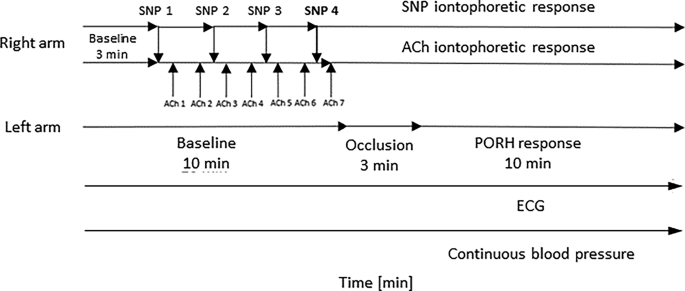
Skin blood flow, electrocardiogram (ECG), and continuous blood pressure monitoring protocol. Skin blood flow was assessed using laser Doppler flowmetry (LDF), ECG was continuously recorded with standard precordial leads, and continuous beat-to-beat blood pressure was monitored using the Finapres NOVA system. SNP – sodium nitroprusside; ACh – acetylcholine; arrows indicate electrical pulses applied during iontophoresis.
After these measurements, the participants randomly underwent either the OGTT or the water loading protocol. The probes remained in the same positions throughout the entire protocol. The protocol was then repeated 45 min and 120 min after the intervention. The 45- and 120-minute time points were selected based on a pilot study in which we defined the time when glucose concentration reached its peak value and returned toward the baseline level, respectively2.
Data processing
The output signals were anonymized and randomized by assigning each study group member a unique code. They were digitized using a DI-4108-E series analog-to-digital converter at a sampling rate of 500 Hz and recorded with a DATAQ Instruments acquisition software (Dataq Instruments, Akron, OH).
Heart rate and Finapres-derived blood pressure assessment
Heart rate was extracted from ECG recordings obtained using a standard lead II configuration. Mean arterial pressure (MAP) was derived from continuous beat-to-beat Finapres recordings. For each inspected time point (0, 45, and 120 min), values were averaged over the first 600 s of ECG and Finapres data.
Raw laser Doppler flux analysis
Raw LD flux values, expressed in absolute perfusion units (PU), were calculated by averaging signals within the same 600-second time intervals later used for wavelet decomposition (the first 600 s of basal forearm LD flux, post-occlusion reperfusion, and the responses to SNP and ACh). This allowed us to assess overall microvascular skin blood flow alongside frequency-specific components.
Wavelet analysis and the cone of influence
To minimize artifacts, LD signals were first filtered using the Hampel filter, which removes only sharp spikes without affecting the physical properties of the signal33. Then, WA was performed using a custom algorithm incorporated into MATLAB, version 9.14, 2023a (The MathWorks Inc., Natick, MA, USA; RRID: SCR_001622).
We opted for a continuous wavelet transform (CWT), which provides a two-dimensional representation of the reconstructed signal in terms of time and frequency (scalogram), offering improved time-frequency resolution compared to the traditional spectral analysis tools. The CWT was numerically implemented as:
$$CWT=\frac{1}{{\sqrt s }}\mathop \sum \limits_{{n=0}}^{{N – 1}} f\left[ n \right]{\psi ^*}\left( {\frac{{n~\Delta t – ~\tau }}{s}} \right)\Delta t,$$
with f [n] representing the discrete samples of the input LD signal, N the total number of discrete samples, Δt the sampling interval of the signal (inverse of the sampling frequency), and ψ the Morlet mother wavelet function, selected to optimize time and frequency localization of the analyzed signal34,35. Scales (s), determining the wavelet’s compression, were spaced logarithmically to ensure adequate resolution across all frequency bands while maintaining computational efficiency, with MATLAB handling this internally. We analyzed the first 600 s of basal forearm LD flux, post-occlusion reperfusion, and responses to SNP and ACh, to capture both the initial transient response and the subsequent stabilization phase.
While traditional recommendations suggest that WA requires relatively long, quasi-stationary signals for reliable results24,25, it is widely recognized that WA’s inherent time-frequency localization properties make it well suited to analyze non-stationary and transient physiological signals36. Building on this foundation, our recent work demonstrates that, when carefully implemented, WA can serve as a sensitive and appropriate tool even for shorter, transient microvascular signals37. These responses, which are difficult to analyze using standard spectral techniques such as FFT due to abrupt amplitude changes, can still yield reliable physiological information through wavelet-based decomposition. By tailoring the analysis window to the physiological duration of interest and applying proper edge correction, we preserve temporal and physiological relevance.
To minimize spectral leakage, which is particularly important in shorter signals, we excluded data outside the cone of influence (COI), defined as the region where wavelet results are unreliable due to edge effects. The data affected by edge effects (i.e., outside the COI) were removed from further calculations using an approximation to the 1/e² rule, an integrated method in MATLAB, to delineate the COI. This approach, recently shown to be essential for reliable WA outcomes in transient LD recordings34, was applied consistently across all responses.
Time-averaged wavelet power spectra were computed, and absolute median power within key frequency intervals was determined for each response. Specifically, we focused on low-frequency endothelial NO-independent (endo NOi) (0.005–0.0095 Hz) and endothelial NO-dependent (endo NOd) (0.0095–0.021 Hz) components, which are presumed to be associated with glucose effects, as well as the myogenic (0.052–0.15 Hz) component, which reflects the intrinsic myogenic activity of VSM cells23 and, as shown later, may also be influenced by glucose loading. Finally, to quantify the impact of each spectral component, the relative power (RP) (the ratio between the absolute median power within the frequency interval of interest and the absolute median power of the total spectrum) was calculated for each test subject from the corresponding power spectra (basal LD flow, PORH, ACh, and SNP).
Heart rate variability
The first 10 min of ECG recordings were analyzed for HRV parameters using Kubios HRV software (Kubios Oy, Kuopio, Finland). To ensure data accuracy, raw ECG signals were pre-processed using automatic beat correction, medium-level automatic noise detection, and artifact removal.
Time-domain parameters, including the standard deviation of normal-to-normal RR intervals (SDNN), presumably reflecting both sympathetic and parasympathetic activity, and root mean square of successive RR interval differences (RMSSD), usually considered a primary indicator of parasympathetic activity20, were calculated. Frequency-domain analysis was performed using FFT to determine low-frequency (LF: 0.04–0.15 Hz) and high-frequency (HF: 0.15–0.4 Hz) power components and the LF/HF ratio. While LF power and LF/HF ratio are often associated with sympathetic modulation, HF power is considered to reflect predominantly parasympathetic activity19.
Statistical analysis
Statistical analysis was performed using IBM SPSS Statistics for Windows, version 29 (IBM Corp., Armonk, N.Y., USA; RRID: SCR_016479). The Shapiro-Wilk test was used to assess normality. Normally distributed variables (e.g., age, cuff-measured blood pressure, MAP, heart rate, glucose levels, logarithmic (ln)-transformed wavelet spectral components, ln-transformed HRV measures) are presented as means with 95% confidence intervals (CIs). Non-normally distributed variables (e.g., body mass index (BMI), room temperature, and relative humidity) are expressed as medians with interquartile ranges (IQR).
Paired t-tests (two-tailed) were used to compare the blood pressure before and after the protocol within and between protocols. A two-way repeated measures analysis of variance (ANOVA) was conducted to assess the effects of the intervention (glucose vs. water) and time (0, 45, and 120 min), both of which were within-subject factors, as well as their interaction on MAP, heart rate, glucose levels, raw LD flux values, wavelet spectral components and HRV metrics.
If the interaction was significant, the simple main effects of time (analyzed using one-way repeated measures ANOVA) and intervention (analyzed using paired t-tests with the Bonferroni correction, denoted as pB) were assessed. A two-sided p-value threshold of 0.05 was used to assess statistical significance. Due to non-normality, the ln-transformed values of some data were used (wavelet powers, RMSSD, SDNN, and LF/HF). Finally, to examine whether the effects of glucose loading were sex-related, sex was included as a between-subject factor in the two-way repeated measures ANOVA model. This approach preserved statistical power by controlling the between-sex variability.
Power calculation
Studies investigating the effects of acute glucose elevation via oral glucose loading on microvascular blood flow in healthy individuals suggest a range of subtle to moderate effects on vascular reactivity4,9. A priori power analysis for repeated measures ANOVA with two conditions (glucose and water loading) and three time points indicated that a sample size of 28 would provide 80% probability of detecting a medium effect (Cohen’s f = 0.25) at α = 0.05, assuming a correlation of r = 0.5 among repeated measures. Calculations were performed using G*Power 3.1 software, version 3.1.9.4 (Heinrich Heine University Düsseldorf, Düsseldorf, Germany; RRID: SCR_013726)38.
link